The goal of PCAtest is to evaluate the overall significance of a PCA, of each PC axis, and of the contributions of each observed variable to the significant axes based on permutation-based statistical tests. PCAtest uses random permutations to build null distributions for several statistics of a PCAanalysis: Psi (Vieira 2012),Phi (Gleason and Staelin 1975), the rank-of-roots (ter Braak 1988), the index of the loadings (Vieira 2012), and the correlations of the PC with the variables (Jackson 1991). Comparing these distributions with the observed values of the statistics, the function tests: (1) the hypothesis that there is more correlational structure among the observed variables than expected by random chance, (2) the statistical significance of each PC, and (3) the contribution of each observed variable to each significant PC. The function also calculates the sampling variance around mean observed statistics based on bootstrap replicates.
Installation
You can install the released (version 0.02) and the development versions from [GitHub] (https://github.com/) with:
# install.packages("devtools")
devtools::install_github("arleyc/PCAtest")
Examples
library(PCAtest)
# PCA analysis of five uncorrelated (r=0) variables
library(MASS)
mu <- rep(0,5)
Sigma <- matrix(c(rep(c(1,0,0,0,0,0),4),1),5)
ex0 <- mvrnorm(100, mu = mu, Sigma = Sigma )
result<-PCAtest(ex0, 100, 100, 0.05, varcorr=FALSE, counter=FALSE, plot=TRUE)
#>
#> Sampling bootstrap replicates... Please wait
#>
#> Calculating confidence intervals of empirical statistics... Please wait
#>
#> Sampling random permutations... Please wait
#>
#> Comparing empirical statistics with their null distributions... Please wait
#>
#> ========================================================
#> Test of PCA significance: 5 variables, 100 observations
#> 100 bootstrap replicates, 100 random permutations
#> ========================================================
#>
#> Empirical Psi = 0.0906, Max null Psi = 0.5364, Min null Psi = 0.0391, p-value = 0.95
#> Empirical Phi = 0.0673, Max null Phi = 0.1638, Min null Phi = 0.0442, p-value = 0.95
#>
#> PCA is not significant!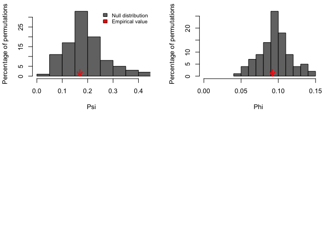
#PCA analysis of five correlated (r=0.25) variables
Sigma <- matrix(c(rep(c(1,0.25,0.25,0.25,0.25,0.25),4),1),5)
ex025 <- mvrnorm(100, mu = mu, Sigma = Sigma )
result<-PCAtest(ex025, 100, 100, 0.05, varcorr=FALSE, counter=FALSE, plot=TRUE)
#>
#> Sampling bootstrap replicates... Please wait
#>
#> Calculating confidence intervals of empirical statistics... Please wait
#>
#> Sampling random permutations... Please wait
#>
#> Comparing empirical statistics with their null distributions... Please wait
#>
#> ========================================================
#> Test of PCA significance: 5 variables, 100 observations
#> 100 bootstrap replicates, 100 random permutations
#> ========================================================
#>
#> Empirical Psi = 1.4947, Max null Psi = 0.4902, Min null Psi = 0.0617, p-value = 0
#> Empirical Phi = 0.2734, Max null Phi = 0.1566, Min null Phi = 0.0555, p-value = 0
#>
#> Empirical eigenvalue #1 = 2.05104, Max null eigenvalue = 1.49457, p-value = 0
#> Empirical eigenvalue #2 = 0.95665, Max null eigenvalue = 1.23612, p-value = 1
#> Empirical eigenvalue #3 = 0.78234, Max null eigenvalue = 1.10792, p-value = 1
#> Empirical eigenvalue #4 = 0.72472, Max null eigenvalue = 0.97997, p-value = 1
#> Empirical eigenvalue #5 = 0.48526, Max null eigenvalue = 0.87503, p-value = 1
#>
#> PC 1 is significant and accounts for 41% (95%-CI:34.5-47.9) of the total variation
#>
#> Variables 2, 3, and 4 have significant loadings on PC 1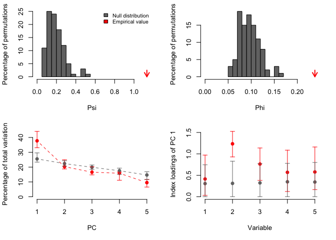
#PCA analysis of five correlated (r=0.5) variables
Sigma <- matrix(c(rep(c(1,0.5,0.5,0.5,0.5,0.5),4),1),5)
ex05 <- mvrnorm(100, mu = mu, Sigma = Sigma )
result<-PCAtest(ex05, 100, 100, 0.05, varcorr=FALSE, counter=FALSE, plot=TRUE)
#>
#> Sampling bootstrap replicates... Please wait
#>
#> Calculating confidence intervals of empirical statistics... Please wait
#>
#> Sampling random permutations... Please wait
#>
#> Comparing empirical statistics with their null distributions... Please wait
#>
#> ========================================================
#> Test of PCA significance: 5 variables, 100 observations
#> 100 bootstrap replicates, 100 random permutations
#> ========================================================
#>
#> Empirical Psi = 4.8505, Max null Psi = 0.6045, Min null Psi = 0.0382, p-value = 0
#> Empirical Phi = 0.4925, Max null Phi = 0.1739, Min null Phi = 0.0437, p-value = 0
#>
#> Empirical eigenvalue #1 = 2.9652, Max null eigenvalue = 1.59307, p-value = 0
#> Empirical eigenvalue #2 = 0.62114, Max null eigenvalue = 1.25937, p-value = 1
#> Empirical eigenvalue #3 = 0.53125, Max null eigenvalue = 1.09766, p-value = 1
#> Empirical eigenvalue #4 = 0.46017, Max null eigenvalue = 0.97471, p-value = 1
#> Empirical eigenvalue #5 = 0.42223, Max null eigenvalue = 0.88145, p-value = 1
#>
#> PC 1 is significant and accounts for 59.3% (95%-CI:51.1-67.2) of the total variation
#>
#> Variables 1, 2, 3, 4, and 5 have significant loadings on PC 1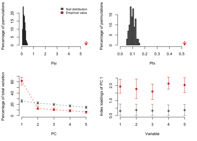
#PCA analysis of seven morphological variables from 29 ant species (from
# Wong and Carmona 2021,  https://doi.org/10.1111/2041-210X.13568)
data("ants")
result<-PCAtest(ants, 100, 100, 0.05, varcorr=FALSE, counter=FALSE, plot=TRUE)
#>
#> Sampling bootstrap replicates... Please wait
#>
#> Calculating confidence intervals of empirical statistics... Please wait
#>
#> Sampling random permutations... Please wait
#>
#> Comparing empirical statistics with their null distributions... Please wait
#>
#> ========================================================
#> Test of PCA significance: 7 variables, 29 observations
#> 100 bootstrap replicates, 100 random permutations
#> ========================================================
#>
#> Empirical Psi = 10.9186, Max null Psi = 2.6398, Min null Psi = 0.6762, p-value = 0
#> Empirical Phi = 0.5099, Max null Phi = 0.2507, Min null Phi = 0.1269, p-value = 0
#>
#> Empirical eigenvalue #1 = 3.84712, Max null eigenvalue = 2.08838, p-value = 0
#> Empirical eigenvalue #2 = 1.52017, Max null eigenvalue = 1.70742, p-value = 0.14
#> Empirical eigenvalue #3 = 0.70634, Max null eigenvalue = 1.3338, p-value = 1
#> Empirical eigenvalue #4 = 0.41356, Max null eigenvalue = 1.14976, p-value = 1
#> Empirical eigenvalue #5 = 0.34001, Max null eigenvalue = 0.96754, p-value = 1
#> Empirical eigenvalue #6 = 0.14515, Max null eigenvalue = 0.72488, p-value = 1
#> Empirical eigenvalue #7 = 0.02765, Max null eigenvalue = 0.63519, p-value = 1
#>
#> PC 1 is significant and accounts for 55% (95%-CI:42.1-65.6) of the total variation
#>
#> Variables 1, 2, 3, 4, 5, and 7 have significant loadings on PC 1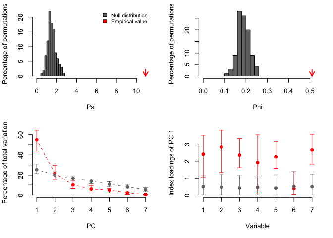
References
Gleason, T. C. and Staelin R. (1975) A proposal for handling missing data. Psychometrika, 40, 229–252.
Jackson, J. E. (1991) A User’s Guide to Principal Components. John Wiley & Sons, New York, USA.
ter Braak, C. F. J. (1990) Update notes: CANOCO (version 3.1). Agricultural Mattematic Group, Report LWA-88-02, Wagningen, Netherlands.
Vieira, V. M. N. C. S. (2012) Permutation tests to estimate significances on Principal Components Analysis. Computational Ecology and Software, 2, 103–123.
Wong, M. K. L. and Carmona, C. P. (2021) Including intraspecific trait variability to avoid distortion of functional diversity and ecological inference: Lessons from natural assemblages. Methods in Ecology and Evolution, 12, 946-957.